Model Training Using ML.NET and TensorFlow - A Comparison

Machine Learning Introduction

Machine learning (ML) is the science (and art) of programming computers so they can learn from data. It is a research field at the intersection of statistics, artificial intelligence, and computer science and is also known as predictive analytics or statistical learning.

Machine learning algorithms have become ubiquitous in everyday life, influencing data-driven research and various scientific problems. They have been applied to recommendations, food ordering, personalized online radio, and recognizing friends in photos. These algorithms have also been applied to understanding stars, discovering new particles, and providing personalized cancer treatments.

Machine Learning Process

The diagram below overviews ML workflow stages. The boxes highlighted in blue describe the processes that manage AI Platform managed services and APIs. In this article, we will limit the discussion to the Train, Evaluate, and Tune stage shown below.

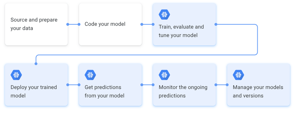
To develop and manage a production-ready model, these are the steps to follow:

Preparing data.
Developing the model.
Training it, evaluating accuracy, and tuning the hyperparameters.
Deploying the model.
Sending prediction requests.
Monitoring, and managing models.

Each step may require re-evaluation and iteratively revisiting the previous steps.

To train a machine learning model, you will need access to a large set of training data that includes features that you wish to predict. Then you can analyze the data, including joining, visualizing, using data-centric languages, identifying features, and cleaning the data to identify anomalous values.

Data preprocessing transforms valid data into the format that best suits the model’s needs, such as normalizing numeric data, applying formatting rules, reducing data redundancy, representing text numerically, and assigning key values to data instances.

Model Training

Machine learning model training involves optimizing tunable parameters in a statistical algorithm to recognize patterns in data and make predictions based on novel data presented.

The accuracy and efficiency of a trained model depend on factors like data quality, model selection, hyperparameter tuning, regularization, evaluation, and deployment. Large Vision and Language Models increase training time exponentially due to their complex architecture and data volume.

Coresets provide an alternative by creating a small, weighted subset of the original input dataset, which has the added advantage of reducing the carbon footprint of ML.

Best Practices in Machine Learning Training

ML model training is essential for accurate, efficient predictions based on input data, requiring careful planning and execution.

Data Preparation

Data preparation is crucial for ML model training, as it significantly impacts performance. High-quality, well-prepared data accurately represents the problem domain.

Hyperparameter Tuning

Hyperparameters are the configuration settings of an ML model that are set before training, such as the learning rate, batch size, and regularization parameters.

Hyperparameters are critical when creating ML models, affecting performance, and requiring careful selection for optimal results.

Hyperparameter tuning involves selecting the optimal hyperparameters for a model, requiring time-consuming, iterative techniques such as:

Grid Search – This technique involves exhaustively searching a predefined range of hyperparameters.
Random Search – This technique selects hyperparameters randomly from a predefined range.
Bayesian Optimization – This technique uses probabilistic models to predict the performance of different hyperparameters and selects the most promising ones for evaluation.

Choosing the Right Model

Selecting the right machine learning model is fundamental to achieving good results. There are various models, such as linear regression, logistic regression, decision trees, random forests, and neural networks.

Each model has its strengths and weaknesses, and the choice depends on the problem’s characteristics.

For Example: Linear regression, logistic regression, decision tree, random forest, or neural networks can be used for predicting continuous values, classifying data into two classes, or classifying data into multiple classes.

Model Regularization

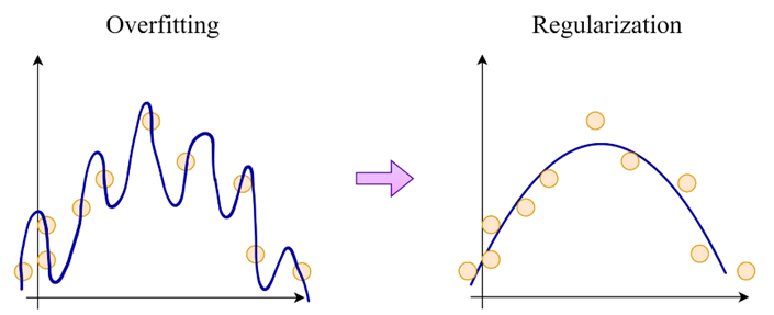
ML models overfit when they perform well on training data but struggle with test data. Regularization prevents overfitting by adding a penalty term.

Model Evaluation

Evaluate the model’s performance after training to ensure accuracy and reliability, comparing it with other methods. Perform the evaluation on a validation dataset, a subset of the training dataset not seen during hyperparameter tuning.

ML models are evaluated using several metrics below:

Accuracy
The accuracy score in machine learning evaluates a model’s number of correct predictions by dividing the number of correct predictions by the total number of predictions.

Precision
Precision is a measure of a machine learning model’s performance, indicating the quality of a positive prediction, calculated by dividing the number of true positives by the total positive predictions.

Recall
Recall, or TPR, is the percentage of data samples a machine learning model correctly classifies as belonging to a “positive class” out of the total samples.

F1 Score
The F1 score is a machine learning evaluation metric that measures a model’s accuracy by combining precision and recall scores across the entire dataset.

AUC-ROC
The AUC-ROC curve measures performance in classification problems, indicating the model’s ability to distinguish between classes. Higher AUC indicates better prediction of 0 and 1 classes, and in the medical field, better distinction between diseased and non-diseased patients.

Analyze model performance on various subsets of validation datasets through cross-validation to ensure optimal performance in all scenarios. A good example is animal classification, where an ML Model is asked to identify a cat from a series of animal pictures.

Model Deployment

The trained and evaluated model is ready for deployment, integrating into the production environment for predictions. Carefully planned and tested, the deployment process ensures model functionality without disruptions. Regular monitoring of performance using techniques like logging, alerts, and dashboards helps identify and address issues.

TensorFlow Keras

Keras is the high-level API for solving machine learning problems on TensorFlow, focusing on deep learning. It covers data processing, hyperparameter tuning, and deployment, offering scalability and cross-platform capabilities. It can be run on TPU Pods or GPU clusters, export models for browsers and mobile devices, and serve Keras models via a web API.

Keras aims to reduce cognitive load by providing simple interfaces, minimizing actions, providing clear error messages, and following progressive disclosure of complexity. It also supports concise code writing.

Keras API Components

Keras’ core data structures consist of layers and models, transforming input/output.

Layers

The tf.keras.layers.Layer class is the fundamental abstraction in Keras, encapsulating state weights and computation. Layers can be trainable or non-trainable, recursively composable, and can handle data preprocessing tasks like normalization and text vectorization. These layers are portable during or after training

Models

A model is an object that groups layers and can be trained on data. Simple models include Sequential, while complex architectures can be built using Keras API or subclassing.

The tf.keras.Model class offers built-in training and evaluation methods, including fit, predict, and evaluate. These methods provide callbacks, distributed training, and step fusing, enabling scaling to multiple GPUs, TPUs, or devices.

ML.NET

ML.NET offers data scientists and developers similar capabilities to the Python ecosystem. Designed for .NET developers, it follows the classic ML pipeline, including data collection, algorithm setting, training, and deployment. It offers a pragmatic programming platform with predefined learning tasks, making it easy to tackle common machine learning scenarios like sentiment analysis, fraud detection, and price prediction.

An ML.NET solution consists of three projects:

An application for a machine learning pipeline.
A class library for data types.
A client application for prediction.

These projects can be defined as the same project for training or consumption.

Model Builder

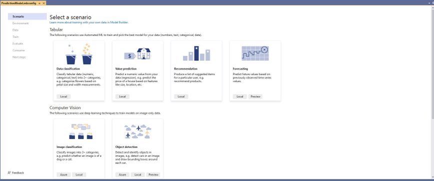
ML.NET Model Builder is a GUI tool for building machine learning models without code. It uses AutoML and deep learning techniques to produce optimal models from data, allowing focus on the desired results.

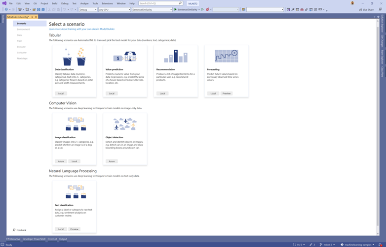
Currently, ML.NET provides several scenarios:

Data classification predicts data points’ categories, values, and recommendations based on features.
Value prediction predicts numeric values.
Recommendation generates personalized recommendations.
Forecasting predicts future trends based on historical data.
Image classification classifies images into predefined categories.
Object detection identifies and localizes multiple objects.
Text classification assigns categories to documents.
Sentence similarity measures the similarity between sentences.

Study Case: Basic Regression

For the study case, we will explore how to build models to predict the fuel efficiency of the late 1970s and early 1980s automobiles.

To do this, we will provide the models with a description of plenty of automobiles from that time. This description includes attributes like cylinders, displacement, horsepower, and weight.

This case is the type of basic regression that aims to predict a specific value. In this example, we will try to predict the total fuel consumption in MPG (Miles Per Gallon) for a particular car model.

Model Training

In this model training, we will use Python for the programming language and TensorFlow Keras. Below are the key steps:

Import the Library

We need to import the related Python libraries for the process. Below is the implementation code in Python:

import matplotlib.pyplot as plt
import numpy as np
import pandas as pd
import seaborn as sns

import tensorflow as tf

from tensorflow import keras
from tensorflow.keras import layers

Loading and Cleaning the Data Set

In this step, we will load the data from the URL and clean it up before it is processed. Below is the implementation in Python:

np.set_printoptions(precision=3, suppress=True)

url = 'http://archive.ics.uci.edu/ml/machine-learning-databases/auto-mpg/auto-mpg.data'
column_names = ['MPG', 'Cylinders', 'Displacement', 'Horsepower', 'Weight',
                'Acceleration', 'Model Year', 'Origin']

raw_dataset = pd.read_csv(url, names=column_names,
                          na_values='?', comment='\t',
                          sep=' ', skipinitialspace=True)
dataset = raw_dataset.copy()
dataset.tail()
dataset.isna().sum()
dataset = dataset.dropna()
dataset['Origin'] = dataset['Origin'].map({1: 'USA', 2: 'Europe', 3: 'Japan'})
dataset = pd.get_dummies(dataset, columns=['Origin'], prefix='', prefix_sep='')
dataset.tail()

Prepare Train and Test Dataset

After the data is ready, we prepare the train and test from the dataset that we prepared. Here is the implementation in Python:

train_dataset = dataset.sample(frac=0.8, random_state=0)
test_dataset = dataset.drop(train_dataset.index)

sns.pairplot(train_dataset[['MPG', 'Cylinders', 'Displacement', 'Weight']], diag_kind='kde')
plt.show()
train_dataset.describe().transpose()

train_features = train_dataset.copy()
test_features = test_dataset.copy()

train_labels = train_features.pop('MPG')
test_labels = test_features.pop('MPG')

Create Regression Model

In this step, we will begin with a single-variable linear regression to predict ‘MPG’ from ‘Horse Power’ There are 2 steps in the single-variable linear regressions:

Use tf.keras.layers to normalize the input characteristics for the “Horsepower.preprocessing” normalization layer.
To create 1 output, apply a linear transformation (y=mx+b) using a linear layer (tf.keras.layers.Dense).

The input_shape option allows us to specify the number of inputs, or it can be determined automatically when the model is run for the first time.

horsepower = np.array(train_features['Horsepower'])

horsepower_normaliser = layers.Normalisation(input_shape=[1,], axis=None)
horsepower_normaliser.adapt(horsepower)

horsepower_model = tf.keras.Sequential([
    horsepower_normaliser,
    layers.Dense(units=1)
])

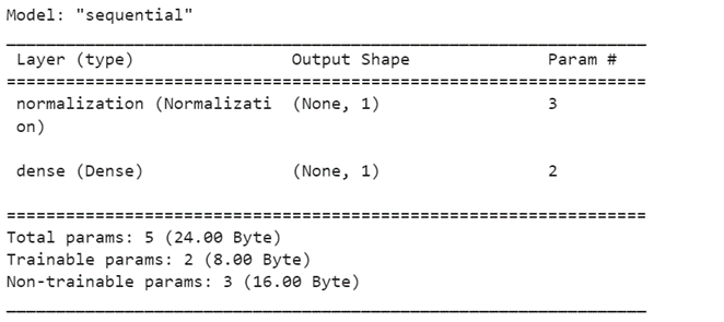
horsepower_model.summary()
horsepower_model.predict(horsepower[:10])

The model above will predict the ‘MPG’ from ‘HorsePower’. Find the detailed output below:

Compiling Model

Compile a model using the compile attribute, specifying the optimizer (SGD, Adam) and the loss function desired for the model. Below is the example usage in Keras:

horsepower_model.compile(
    optimizer=tf.keras.optimizers.Adam(learning_rate=0.1),
    loss='mean_absolute_error')

Fitting the Model

Fitting a model on split training data allows for the use of parameters like epochs, verbose, and validation split.

history = horsepower_model.fit(
    train_features['Horsepower'],
    train_labels,
    epochs=100,
    # Suppress logging.
    verbose=0,
    # Calculate validation results on 20% of the training data.
    validation_split = 0.2)

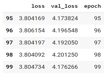
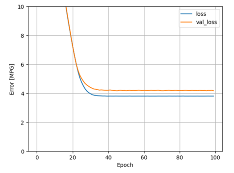
Let’s visualize the model’s training progress using the stats stored in the history object:

hist = pd.DataFrame(history.history)
hist['epoch'] = history.epoch
hist.tail()

def plot_loss(history):
  plt.plot(history.history['loss'], label='loss')
  plt.plot(history.history['val_loss'], label='val_loss')
  plt.ylim([0, 10])
  plt.xlabel('Epoch')
  plt.ylabel('Error [MPG]')
  plt.legend()
  plt.grid(True)

plot_loss(history)

Predicting the Output

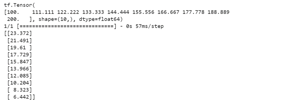
The model is now ready for us to predict the output. Let’s use random test data to predict the output.

x = tf.linspace(100, 200, 10)
print(x)
y = horsepower_model.predict(x)
print(y)

Here is the result:

Model Training Using ML.NET

In this Model Training, we’ll use the model builder to develop the prediction model and a similar dataset to the previous section.

Prepare the Data Set

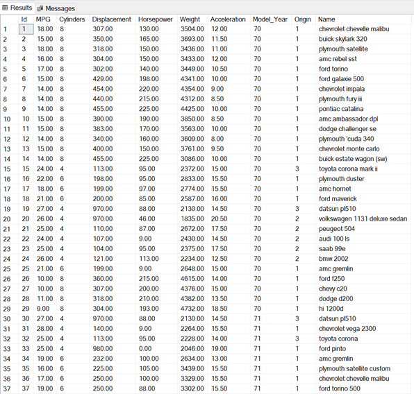
For the data set, we will download the data from http://archive.ics.uci.edu/ml/machine-learning-databases/auto-mpg/auto-mpg.data then clean up the data and export them into the SQL Server table.

Below is the example result:

Setup ML.NET Project

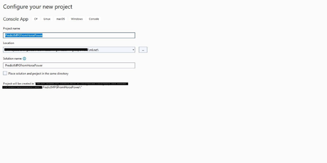
In this study case, we will use Visual Studio 2022 with the ML.NET Extension installed. Once it is installed, we can start creating the project. The project can be of any type, in this study case, we will use a simple console project.

Add ML Model to the Project

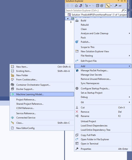
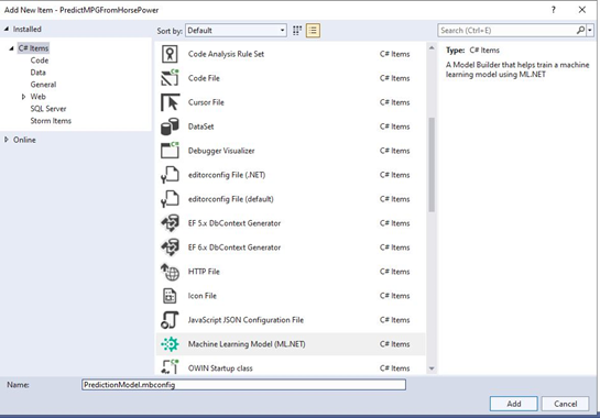
The next step is adding the ML.NET Model to the Project that we’ve created before. We can consider this process a success when we can see the ML.NET Scenarios Page.

Training the Model

Once we’re ready we can start the training process. Below are the detailed steps.

Select the correct scenario. For this scenario, select Value Prediction.

Select the training environment.

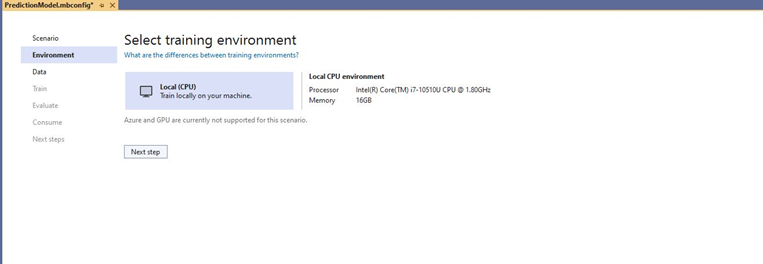
In this training, we’ll use the local resources (CPU). Other environments are Azure and GPU. For GPU, we need to set up the hardware first before we can use it. For now, let’s use the CPU.

Add the Data

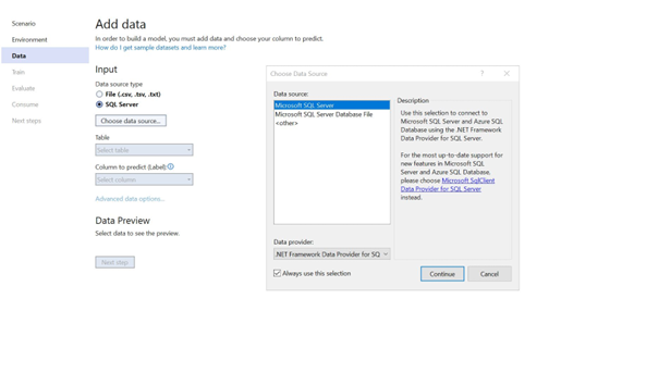
The next step is adding the dataset. Since we are using SQL Server then we will select SQL Server as the data source.

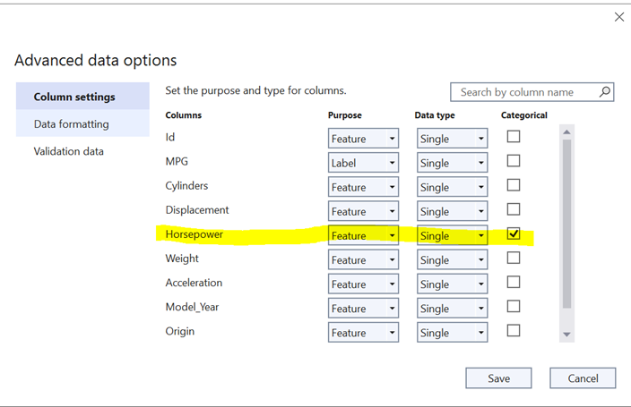
Then we also need to select the Label column. In this case, we will use ‘MPG’ as the Label as above.

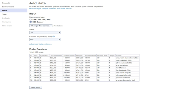
After selecting the label, we need to select the feature. For this feature we will use ‘Horsepower’.

Conduct Training Process

Once everything is ready, we can start the training process. The model builder allows us to specify the time required to train the model. This will depend on the number of records that we’d like to train. Since the dataset is small let us set the time to 60 seconds. Since we are using Auto ML, we do not have to worry about selecting the wrong algorithm for the model. The Auto ML will simply select it for us.

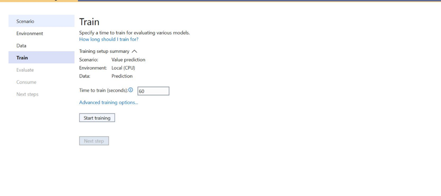
Below is the output from the training:

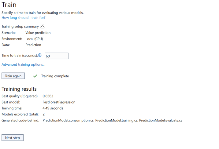
Consume the Model in the Console Application

To test the prediction process, we will consume the model into the console application.

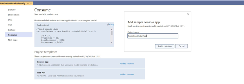
Let’s use the console app to predict our test data.

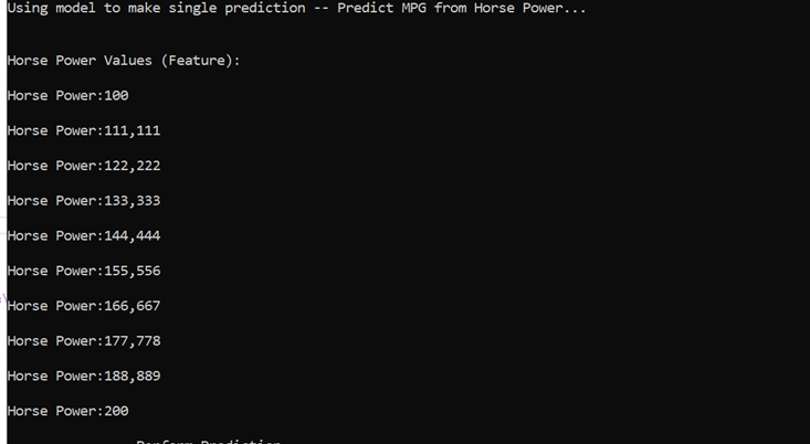
Run the prediction and here is the result.

Conclusions

The main step in the machine learning pipeline is model training. The better the output model, the better the machine learning process outcome, since the model must be used by the program which will define the application’s output. Therefore, the developer’s choice of Machine Learning Framework is essential.

TensorFlow Keras is a well-known, well-tested framework that is used by many developers since it is open source, has excellent documentation, a sizable community behind it, and is utilized all over the world. The basic framework, however, doesn’t directly support the CPU and necessitates modification to create a high-precision model. TensorFlow Keras is intended for more advanced users.

On the other hand, ML.NET is a replacement for the Machine Learning Framework that offers Model Builder and Auto ML that simplify the training process. Even if a developer has no experience with machine learning, they will find it easy to adapt because it is built on top of the .Net Framework. The developer can choose the optimum method with the highest level of model output accuracy by using auto ML. Additionally, configuring ML.NET to run on CPU or GPU is simpler.

ML.NET is an excellent choice for people who are starting their journey into Machine Learning as it offers many tools that simplify the development of the model (Model Builder and Auto ML). It also provides the TensorFlow Model Utilization feature, which is a useful alternative for developers who have developed models on top of TensorFlow libraries in the past.

References

“Introduction to Machine Learning” by Dino Esposito, Francesco Esposito

https://www.tensorflow.org/tutorials/keras

https://www.projectpro.io/recipes/perform-basic-regression-keras-model

https://neptune.ai/blog/fighting-overfitting-with-l1-or-l2-regularization

Author: Zainal Arifin, Technology Evangelist